A Brief Intro to Gibbs Sampling
Posted on September 03, 2015
For statistical inference, Gibbs Sampling is commonly used, especially in Baysian Inference. It is a Markov Chain Monte Carlo (MCMC) algorithm for obtaining a sequence of observations when directly sampling from a multivariate probability distribution is difficult. Since it is an randomized algorithm, the result produced each time may be different.
Why we need Gibbs Sampling? When the joint distribution is unknown and it is very difficult to sample from the distribution directly, but the conditional distribution of each random variable is known and could be easy to sample from, then one can take samples from conditional distribtuion of each variable. After thousands times of sampling, a markov chain constituted by the sequences of samples can be obtained, and stationary distribution of the chain is just the joint distribution we are seeking.
Gibbs sampling generates a Markov Chain of samples so that each sample is correlated with nearby samples. Therefore, if independent random samples are desired, one must pay attention to use this method. Moreover, samples in the burn-in period generated by Gibbs sampling may not accurately represent the desired distributions.
If one want to get \(K\) samples of from a joint distribution , let \(i\)th sample is denoted by , the procedure of Gibbs Sampling is:
(1) Begin with some initial value \(\mathbf{X^{(0)}}\).
(2) Sample each component variable \(x_{j}^{(i+1)}\) from the distribution of that varibale conditioned on all other variables.
(3) Repeat the above step \(K\) times.
Following is an example Python program for Gibbs Sampling.
Considering BivariateNormal distrbition case, we define a new function gibbs to make Gibbs Sampling:
import numpy as np
import scipy
from matplotlib.pyplot import *
from scipy import *
from scipy import stats
from bvn import BivariateNormal, plot_bvn_rho,plot_bvn

def gibbs(bvn, n):
    gibbs_sample = []
    x_initial, y_initial = 5., 5
    # Set initial start point.
    xx = x_initial
    yy = y_initial

    for i in range(n):
        u = stats.uniform.rvs(loc = 0,scale = 1, size = 1 )
        # Throw a coin to decide which variable to be updated.

        if u > 0.5 :
            # Only update x if u > 0.5
            x_new = bvn.x_y_sample(yy)
            xx = x_new
            pair = [xx, yy]
        else:
            # Only update y if u < 0.5
            y_new = bvn.y_x_sample(xx)
            yy = y_new
            pair = [xx,yy]
        gibbs_sample += [pair]

    return gibbs_sample
(Note: Before using the Gibbs Sampling program shown above, one must create a new class bvn which contains BivariateNormal methods and plot_bvn_rho,plot_bvn methods. This class can be found in my GitHub)
Set the correlation between the two random variables as \(\rho = 0.5\) and marginal mean, variance, we generate 400 samples.
rho = 0.5 # Set rho = 0.5 to make Gibbs Sampling.
# Set a bivariate normal distribution of (x,y) first.
mu_x, mu_y, sig_x, sig_y = 0.,0.,1.,1.
means = array([mu_x, mu_y])
sigs = array([sig_x, sig_y])
bvn = BivariateNormal(means, sigs, rho)

n = 400 # The size of sampling.
sampleOne = gibbs(bvn, n)
Then we plot the theoretical BivariateNormal distribution and our samples generated by Gibbs Sampling.
xxx = [sampleOne[i][0] for i in range(len(sampleOne))] # Samples of x.
yyy = [sampleOne[i][1] for i in range(len(sampleOne))] # Samples of y.
plot_bvn(rho)
plot(xxx,yyy,ls = '--',marker = 'o',
markerfacecolor = 'red', markersize = 3)
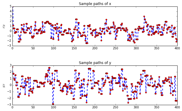
subplots(nrows = 2, ncols = 1, figsize = (10,6))
subplots_adjust(hspace = 0.5)
subplot(211)
plot(xxx,ls = '--',lw = 2, marker = 'o',
markerfacecolor = 'red', markersize = 5)
title("Sample paths of x")
ylabel('$x|y$')
xlim([0,float(n)])
subplot(212)
plot(yyy,ls = '--',lw = 2, marker = 'o',
markerfacecolor = 'red', markersize = 5)
title("Sample paths of y")
ylabel('$y|x$')
xlim([0,float(n)])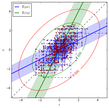
As an comparison, we set the correlation between two random variables as 0.97, then see what will happen.
rho = 0.97 # Set rho = 0.5 to make Gibbs Sampling.
# Set a bivariate normal distribution of (x,y) first.
mu_x, mu_y, sig_x, sig_y = 0.,0.,1.,1.
means = array([mu_x, mu_y])
sigs = array([sig_x, sig_y])
bvn = BivariateNormal(means, sigs, rho)

n = 400 # The size of sampling.
sampleTwo = gibbs(bvn, n)
xxx = [sampleTwo[i][0] for i in range(len(sampleTwo))] # Samples of x.
yyy = [sampleTwo[i][1] for i in range(len(sampleTwo))] # Samples of y.
plot_bvn(rho)
plot(xxx,yyy,ls = '--',marker = 'o',
markerfacecolor = 'red', markersize = 3)
subplots(nrows = 2, ncols = 1, figsize = (10,6))
subplots_adjust(hspace = 0.5)
subplot(211)
plot(xxx,ls = '--',lw = 2, marker = 'o',
markerfacecolor = 'red', markersize = 5)
title("Sample paths of x")
ylabel('$x|y$')
xlim([0,float(n)])
subplot(212)
plot(yyy,ls = '--',lw = 2, marker = 'o',
markerfacecolor = 'red', markersize = 5)
title("Sample paths of y")
ylabel('$y|x$')
xlim([0,float(n)])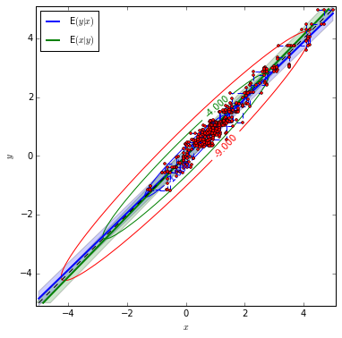
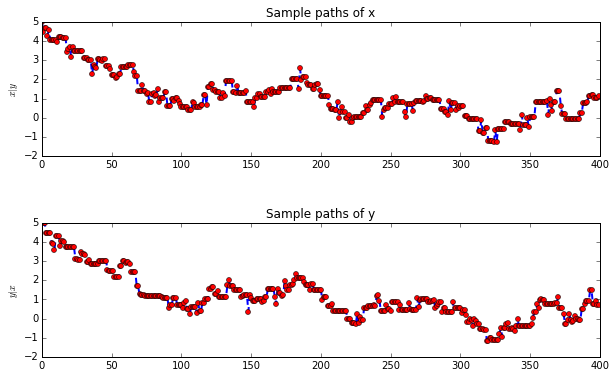
According to sample paths figures, it is indicated that when the correlation between x and y is small, the sample paths look much more like random. With \(\rho=0.97\), the sample paths seem highly correlated.