Data Analysis & Quant. Finance
A Brief Intro to Gibbs Sampling
September 03, 2015
For statistical inference, Gibbs Sampling is commonly used, especially in Baysian Inference. It is a Markov Chain Monte Carlo (MCMC) algorithm for obtaining a sequence of observations when directly sampling from a multivariate probability distribution is difficult. Since it is an randomized algorithm, the result produced each time may be different.
Why we need Gibbs Sampling? When the joint distribution is unknown and it is very difficult to sample from the distribution directly, but the conditional distribution of each random variable is known and could be easy to sample from, then one can take samples from conditional distribtuion of each variable. After thousands times of sampling, a markov chain constituted by the sequences of samples can be obtained, and stationary distribution of the chain is just the joint distribution we are seeking.
Gibbs sampling generates a Markov Chain of samples so that each sample is correlated with nearby samples. Therefore, if independent random samples are desired, one must pay attention to use this method. Moreover, samples in the burn-in period generated by Gibbs sampling may not accurately represent the desired distributions.
If one want to get \(K\) samples of from a joint distribution , let \(i\)th sample is denoted by , the procedure of Gibbs Sampling is:
(1) Begin with some initial value \(\mathbf{X^{(0)}}\).
(2) Sample each component variable \(x_{j}^{(i+1)}\) from the distribution of that varibale conditioned on all other variables.
(3) Repeat the above step \(K\) times.
Following is an example Python program for Gibbs Sampling.
Considering BivariateNormal distrbition case, we define a new function gibbs to make Gibbs Sampling:
import numpy as np
import scipy
from matplotlib.pyplot import *
from scipy import *
from scipy import stats
from bvn import BivariateNormal, plot_bvn_rho,plot_bvn

def gibbs(bvn, n):
    gibbs_sample = []
    x_initial, y_initial = 5., 5
    # Set initial start point.
    xx = x_initial
    yy = y_initial

    for i in range(n):
        u = stats.uniform.rvs(loc = 0,scale = 1, size = 1 )
        # Throw a coin to decide which variable to be updated.

        if u > 0.5 :
            # Only update x if u > 0.5
            x_new = bvn.x_y_sample(yy)
            xx = x_new
            pair = [xx, yy]
        else:
            # Only update y if u < 0.5
            y_new = bvn.y_x_sample(xx)
            yy = y_new
            pair = [xx,yy]
        gibbs_sample += [pair]

    return gibbs_sample
(Note: Before using the Gibbs Sampling program shown above, one must create a new class bvn which contains BivariateNormal methods and plot_bvn_rho,plot_bvn methods. This class can be found in my GitHub)
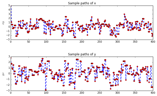
Set the correlation between the two random variables as \(\rho = 0.5\) and marginal mean, variance, we generate 400 samples.
rho = 0.5 # Set rho = 0.5 to make Gibbs Sampling.
# Set a bivariate normal distribution of (x,y) first.
mu_x, mu_y, sig_x, sig_y = 0.,0.,1.,1.
means = array([mu_x, mu_y])
sigs = array([sig_x, sig_y])
bvn = BivariateNormal(means, sigs, rho)

n = 400 # The size of sampling.
sampleOne = gibbs(bvn, n)
Then we plot the theoretical BivariateNormal distribution and our samples generated by Gibbs Sampling.
xxx = [sampleOne[i][0] for i in range(len(sampleOne))] # Samples of x.
yyy = [sampleOne[i][1] for i in range(len(sampleOne))] # Samples of y.

plot_bvn(rho)
plot(xxx,yyy,ls = '--',marker = 'o',
     markerfacecolor = 'red', markersize = 3)


subplots(nrows = 2, ncols = 1, figsize = (10,6))
subplots_adjust(hspace = 0.5)
subplot(211)
plot(xxx,ls = '--',lw = 2, marker = 'o',
     markerfacecolor = 'red', markersize = 5)
title("Sample paths of x")
ylabel('$x|y$')
xlim([0,float(n)])
subplot(212)
plot(yyy,ls = '--',lw = 2, marker = 'o',
     markerfacecolor = 'red', markersize = 5)
title("Sample paths of y")
ylabel('$y|x$')
xlim([0,float(n)])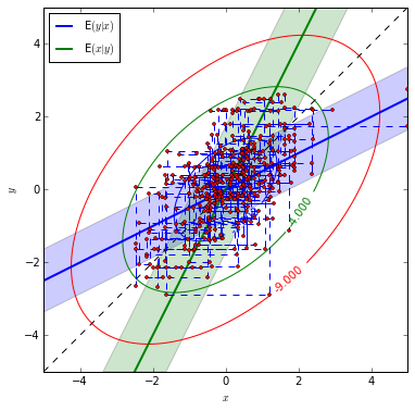
As an comparison, we set the correlation between two random variables as 0.97, then see what will happen.
rho = 0.97 # Set rho = 0.5 to make Gibbs Sampling.
# Set a bivariate normal distribution of (x,y) first.
mu_x, mu_y, sig_x, sig_y = 0.,0.,1.,1.
means = array([mu_x, mu_y])
sigs = array([sig_x, sig_y])
bvn = BivariateNormal(means, sigs, rho)

n = 400 # The size of sampling.
sampleTwo = gibbs(bvn, n)
xxx = [sampleTwo[i][0] for i in range(len(sampleTwo))] # Samples of x.
yyy = [sampleTwo[i][1] for i in range(len(sampleTwo))] # Samples of y.
plot_bvn(rho)
plot(xxx,yyy,ls = '--',marker = 'o',
markerfacecolor = 'red', markersize = 3)
subplots(nrows = 2, ncols = 1, figsize = (10,6))
subplots_adjust(hspace = 0.5)
subplot(211)
plot(xxx,ls = '--',lw = 2, marker = 'o',
markerfacecolor = 'red', markersize = 5)
title("Sample paths of x")
ylabel('$x|y$')
xlim([0,float(n)])
subplot(212)
plot(yyy,ls = '--',lw = 2, marker = 'o',
markerfacecolor = 'red', markersize = 5)
title("Sample paths of y")
ylabel('$y|x$')
xlim([0,float(n)])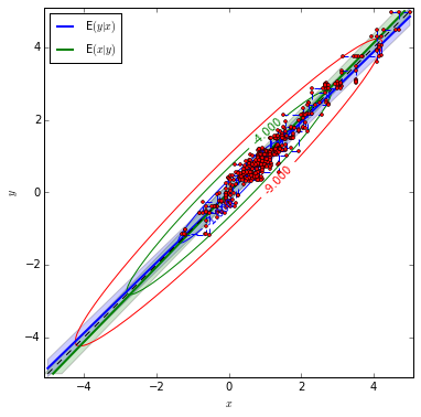
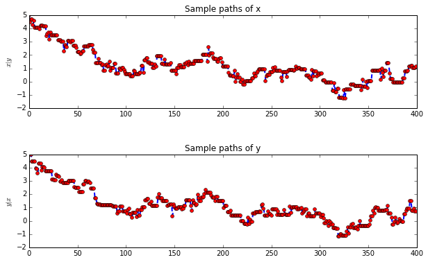
According to sample paths figures, it is indicated that when the correlation between x and y is small, the sample paths look much more like random. With \(\rho=0.97\), the sample paths seem highly correlated.
Crawling and Storing Data with R and MySQL
August 15, 2015
In this article, I am going to talk about how to crawl data from Internet with R, and then store the data into MySQL database.
When someone conducts quantitative analysis on financial markets, data is an imperative element. Beside using Bloomberg, DataStream or some other tools to get data, we can also crawl data from various website, especially when the data you need are displayed on different pages, e.g, daily closed prices of stocks contained in the S&P 500 from 2001-01-01 to 2015-08-01, which are often displayed on multi pages. Stock prices can be easily found on the Yahoo Finance. However, if downloading data from stock to stock, one needs to open more 500 pages and copy these data repetitively. If this work is finished manually, it will be very time-consuming. Therefore, crawling technique can be very efficient.
Taking crawling trading information of stocks contained in the S&P 500 as the example:
library(rvest)
library(pipeR)
library(sqldf)

html <- html('https://en.wikipedia.org/wiki/List_of_S%26P_500_companies')

title = html_nodes(html,xpath = '//table/tr[1]/th')
title_text = html_text(title)[1:7]
title_text
#
# [1] "Ticker symbol"           "Security"
# [3] "SEC filings"             "GICS Sector"
# [5] "GICS Sub Industry"       "Address of Headquarters"
# [7] "Date first added"
#

# Calculate the number of stocks contained in S&P 500
number = length(html_nodes(html,xpath = '//table[1]/tr/td[1]'))
sp500_stocks = data.frame(number = c(1:number))

# extract info from the table in wiki website.
sp500_stocks['Ticker_Symbol'] = html_nodes(html,xpath = '//table[1]/tr/td[1]') %>>%
  html_text()

sp500_stocks[,'Security'] = html_nodes(html,xpath = '//table[1]/tr/td[2]') %>>%
  html_text()

sp500_stocks['SEC_filings'] = html_nodes(html,xpath = '//table[1]/tr/td[3]') %>>%
  html_text()

sp500_stocks['GICS_Sector'] = html_nodes(html,xpath = '//table[1]/tr/td[4]') %>>%
  html_text()

sp500_stocks['GICS_Sub_Industry'] = html_nodes(html,xpath = '//table[1]/tr/td[5]') %>>%
  html_text()

sp500_stocks['Address_of_Headquarters'] = html_nodes(html,xpath = '//table[1]/tr/td[6]') %>>%
  html_text()

sql = "SELECT * FROM sp500_stocks
ORDER BY Ticker_Symbol"

sp500_stocks = sqldf(sql)
Since we have already get all the symbols of stocks listed in S\&P500 index, the next step is to find the data we need on the Internet and parse the websites then crawling all the information we need. Taking crawling stock price data from Yahoo Finance as exmaple:
setwd("~/Desktop/Data")

library(rvest)
library(stringr)
library(pipeR)
library(data.table)


sp500_stocks <- read.csv('sp500_stock_list.csv')
stockList <- sp500_stocks[,3:4]

# Create a data frame to hold all the stock data.
allStockData <- data.frame(Date = 0, Open = 0,
                           High = 0, Low = 0,
                           Close = 0, Volume = 0,
                           Adj_Close = 0, Symbol = 'a',
                           Security = 'a')

for(i in 1:length(stockList[,1])){

  html <- sprintf("http://real-chart.finance.yahoo.com/table.csv?s=%s&a=00&b=2&c=1962&d=06&e=23&f=2015&g=d&ignore=.csv",stockList[i,1])
  stockData <- html(html) %>>%
    html_node(xpath = "//p") %>%
    html_text() %>%
    strsplit("\n") %>%
    unlist()

  # Create a data frame to store the data.
  n = length(stockData)
  temp_df <- data.frame(Date = rep(0,n), Open = rep(0,n),
                        High = rep(0,n), Low = rep(0,n),
                        Close = rep(0,n), Volume = rep(0,n),
                        Adj_Close = rep(0,n))
  for (j in 2:n){
    temp_df[j,] = unlist(strsplit(stockData[j],','))
    #     temp_df[i,1] = unlist(strsplit(temp[i],','))[1]
    #     temp_df[i,2] = unlist(strsplit(temp[i],','))[7]
  }
  temp_df = temp_df[-1,]
  temp_df['Symbol'] = stockList[i,1]  # First column is symbol
  temp_df['Security'] = stockList[i,2] # Second column is security name

  allStockData = rbind(temp_df, allStockData)
}


write.csv(allStockData, file = 'SP500_All_Stock_Data.csv')
After crawling all the data required, one can try to connect database with R. RMySQL is a powerful package that can connect R with database and manipulate data directly in R. Followings are some basic instructions of using MySQL in R.
library(RMySQL)
library(pipeR)

conn <- dbConnect(MySQL(),
                  dbname = "stockdb",
                  username = "stockdata",
                  password = "testpassword")

# write data frame into database.
dbWriteTable(conn, 'sp500_stockdata', allStockData, row.names=F, append=F, overwrite = T)

sql2 <-"SELECT * FROM stockdb.sp500_stockdata
WHERE symbol = 'AAPL'
limit 50"

# execute a simple query statement. And all the fetched data are stored as a data frame.
queryTable2 <- dbSendQuery(conn, sql2) %>>%
  dbFetch()

queryTable


dbListTables(conn)
dbSendQuery(conn, 'drop table sp500_stockdata2;')
dbDisconnect(conn)

dbClearResult()Connect to MySQL with Python
July 25, 2015
##Connect to MySQL with Python in MAC
Installation environment: OS X Yosemite, Python 2.7.9
The official API MySQLdb is contained in the package MySQL-python. Therefore, when using pip to install the MySQLdb, just simply execute the command in Terminal:pip install MySQL-python.
Solve an error Reason: image not found
After installing the MySQL-python successfully, let’s import this package in the Python to connect to MySQL database. However, an error as follows may occur:
 >>> import MySQLdb
 /Library/Python/2.7/site-packages/MySQL_python-1.2.3-py2.7-macosx-10.7-intel.egg/_mysql.py:3: UserWarning: Module _mysql was already imported from /Library/Python/2.7/site-packages/MySQL_python-1.2.3-py2.7-macosx-10.7-intel.egg/_mysql.pyc, but /Users/***/Downloads/MySQL-python-1.2.3
 is being added to sys.path
Traceback (most recent call last):
  File "<stdin>", line 1, in <module>
  File "MySQLdb/__init__.py", line 19, in <module>
    import _mysql
  File "build/bdist.macosx-10.7-intel/egg/_mysql.py", line 7, in <module>
  File "build/bdist.macosx-10.7-intel/egg/_mysql.py", line 6, in __bootstrap__
ImportError: dlopen(/Users/***/.python-eggs/MySQL_python-1.2.3-py2.7-macosx-10.7-intel.egg-tmp/_mysql.so, 2): Library not loaded: libmysqlclient.18.dylib
  Referenced from: /Users/***/.python-eggs/MySQL_python-1.2.3-py2.7-macosx-10.7-intel.egg-tmp/_mysql.so
  Reason: image not found
Don’t worry. The solution is easy. Just open the terminal and execute command:
> sudo ln -s /usr/local/mysql/lib/libmysqlclient.18.dylib /usr/lib/libmysqlclient.18.dylib

> sudo ln -s /usr/local/mysql/lib /usr/local/mysql/lib/mysql
Then re-open your Python and import the package again, I think the problem will probably be solved. Yeah! :)